13. Balanced Trees

1. Videos

There is are two videos that covers the material in this notes. The link to the page with vides is: Videos about trees, sets, and maps

2. Balanced binary search tree

Binary search tree is balanced if the heights of left and right sub-trees are approximately the same. We will specify later what the word approximately means.

If a tree is balanced, then it can have a relatively small height, and yet store a lot of nodes. Let us first define the size of the tree and the height of the tree.

If we denote by \(N\) the total number of nodes, and by \(h\) the height of the tree, for balanced tree we can have \(N\approx 2^h\), or eqiuvalently, \(h\approx \log(N)\).

When we search a tree, we always start from the root. In each step we always go down. Therefore, the search takes at most \(h\) steps. If the tree is balanced, the search takes at most \(O(\log N)\) steps.

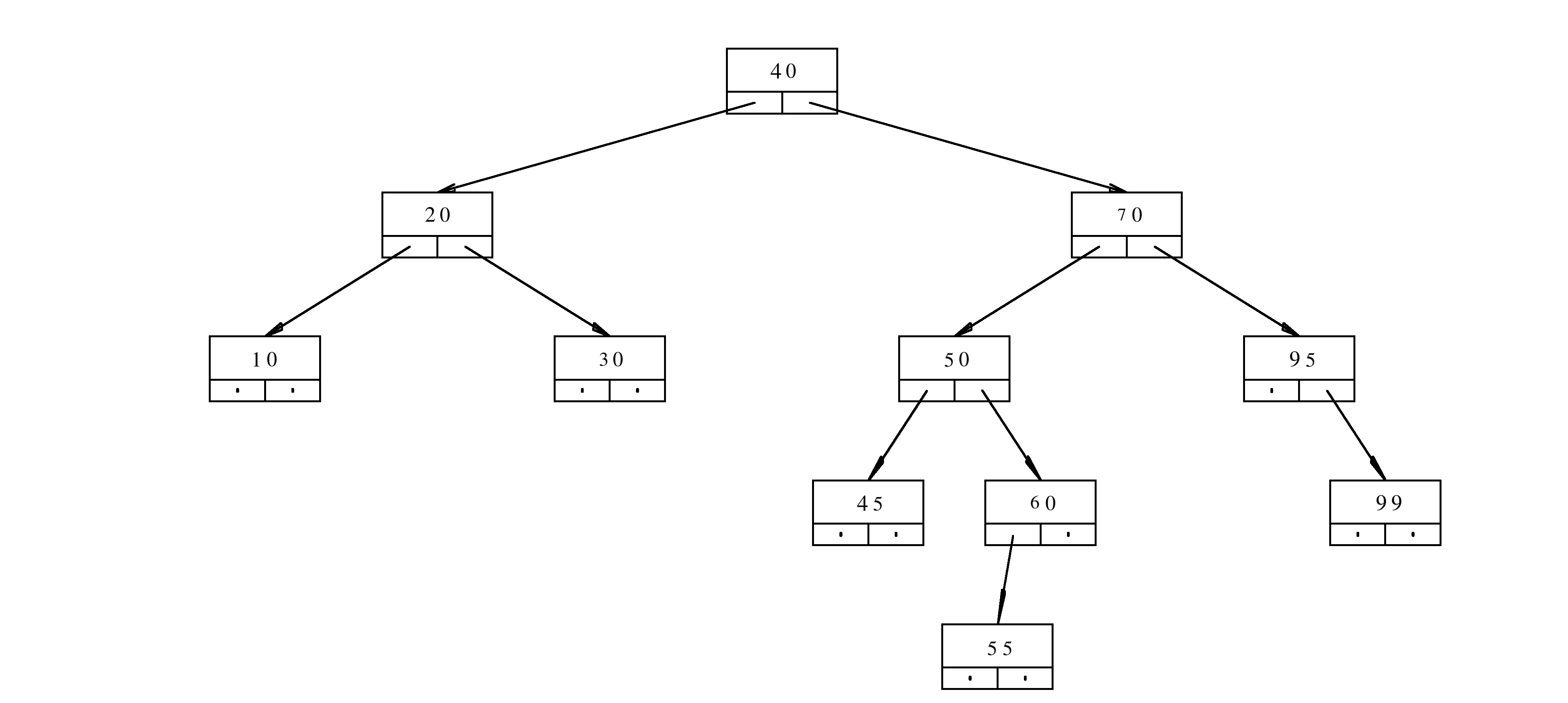
We built some simple trees in previous lecture notes. These trees were not perfect. If the data were sorted before insertion, then the tree would turn into a linked list. Inserting, deleting, and searching would be long operations. The complexity of the operations would be \(O( N)\), because if the tree is deformed and turned into a linked list, then the size \(N\) and the height \(h\) are the same. The search would take \(h\) steps. However, since \(h\) is the same as \(N\), the searching for elements in these unfortunate trees would take \(N\) steps.

3. AVL Trees

Fortunately, there are algorithms that can keep the trees balanced. There are several ways to construct balanced trees, and in each of these ways, the definition of balanced is slightly different. However, each of these trees comes with algorithms for insertion and removal of the elements. Each of these algorithms has its own constant \(C\) such that:

The first such algorithm, and the one that is the easiest to explain, is the AVL algorithm. The algorithm was discovered by Georgy Adelson-Velsky and Evgenii Landis in 1962.

The AVL tree is defined in the following way.

Each node of AVL tree contains two additional attributes: The height of the left sub-tree and the height of the right sub-tree.

The insertion and removal are performed in two stages:

• Stage 1. Insert (remove) the node just as you would do for a regular binary search tree. Update the heights as necessary in all of the nodes along the path that was traveled during the insertion or removal.
• Stage 2. Inspect whether the balance was ruined. If it was, then re-balance the tree.

The stage 1 takes at most \(O(\log N)\) steps. The stage 2 also takes at most \(O(\log N)\) steps. Therefore, each insertion and each removal takes at most \(2\cdot O(\log N)=O(\log N)\) steps.

4. AVL rotations

The re-balance is not too difficult to implement. If a single node is inserted or deleted, there are very few possible ways in which the balance can be ruined. Since we started with an AVL tree, one single insertion or one single removal cannot shake the tree too much out of balance.

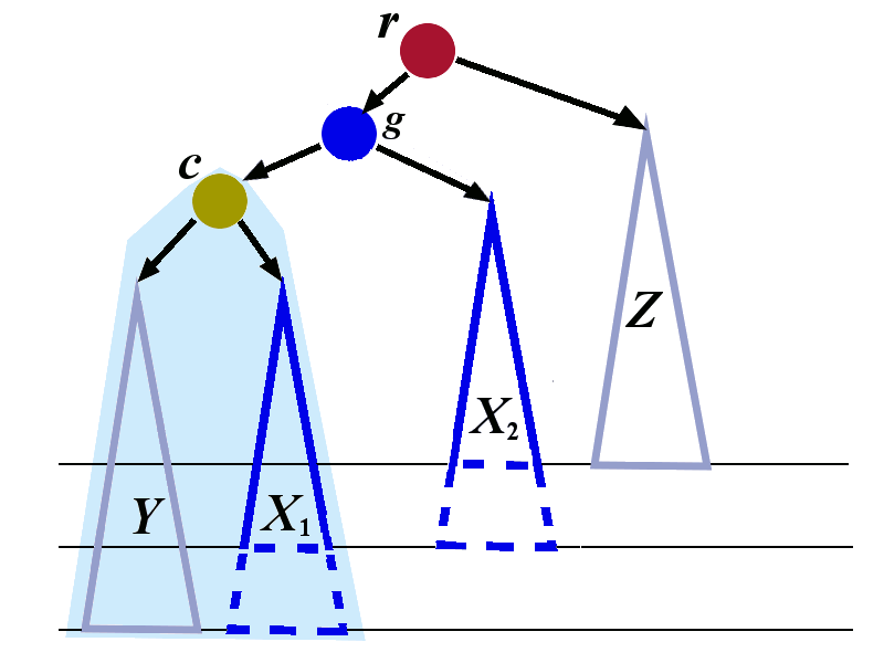
We identify the lowest node that violates the AVL property. We denote this node by \(r\). The node \(r\) has two children. Each child is a root of a sub-tree. One of the sub-tree has height that is by \(2\) bigger than the height of the other sub-tree. We will denote by \(c\) the child whose sub-tree is bigger. We will denote by \(X\) and \(Y\) the two sub-trees of \(c\). Denote by \(Z\) the sub-tree of the sibling of \(c\).

4.1. Single rotations

The easiest cases are shown in the picture below.

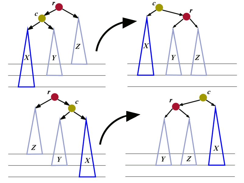
There are four pictures in total. The pictures on the left are showing two cases where the trees are out of balance. In each of the two cases we can perform 3 re-assignments of pointers to restore the balance.

Let us analyze the unbalanced tree at the top:

• 1. The pointer r->aLeft should be changed. It should stop pointing to c. Instead, it should point to the root of the sub-tree \(Y\).
• 2. The pointer c->aRight should be changed from \(Y\) to r.
• 3. The pointer from the parent of r should be changed to point to c.

The combination of the previous 3 operations is called right rotation. The root r moves to become the right child of its former child.

In an analogous way we construct the left rotation to restore the balance of the tree shown at the bottom.

4.2. Double rotations

We now consider the cases in which the taller sub-tree of the child \(c\) is inside. One such case is shown in the left picture below.

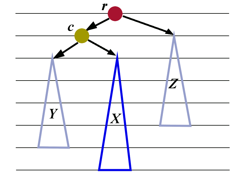
The child \(c\) is the left child of \(r\). The child \(c\) has two sub-trees: \(Y\) and \(X\). The right sub-tree \(X\) is taller than the left sub-tree \(Y\).

An analogous situation would be if \(c\) is the right child whose left sub-tree is taller than the right sub-tree.

The balance to the tree can be restored by performing two rotations that were already constructed in Subsection 4.1.

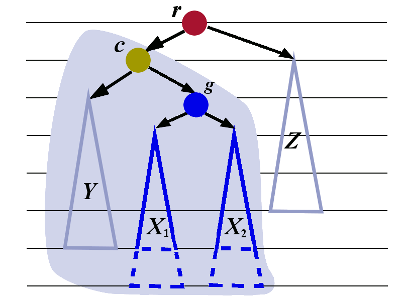
We need to introduce some additional labels. We first look at the tree \(X\) and give the name \(g\) to its root. We give the names \(X_1\) and \(X_2\) to the sub-trees of \(g\). The letter \(g\) was chosen because it stands for grandchild. The node \(g\) is the grandchild of \(r\).

We now apply the left-rotation to the tree whose root is \(g\). The transformation is shown in the picture below.

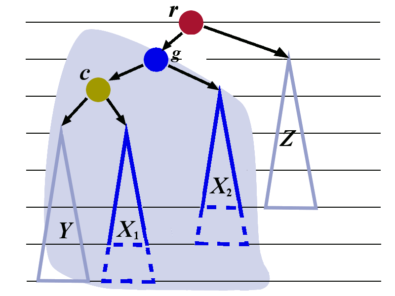
We now perform the right rotation to the tree whose root is \(r\). The transformation is shown below. The tree with root \(c\) is treated as a single tree in this right rotation..

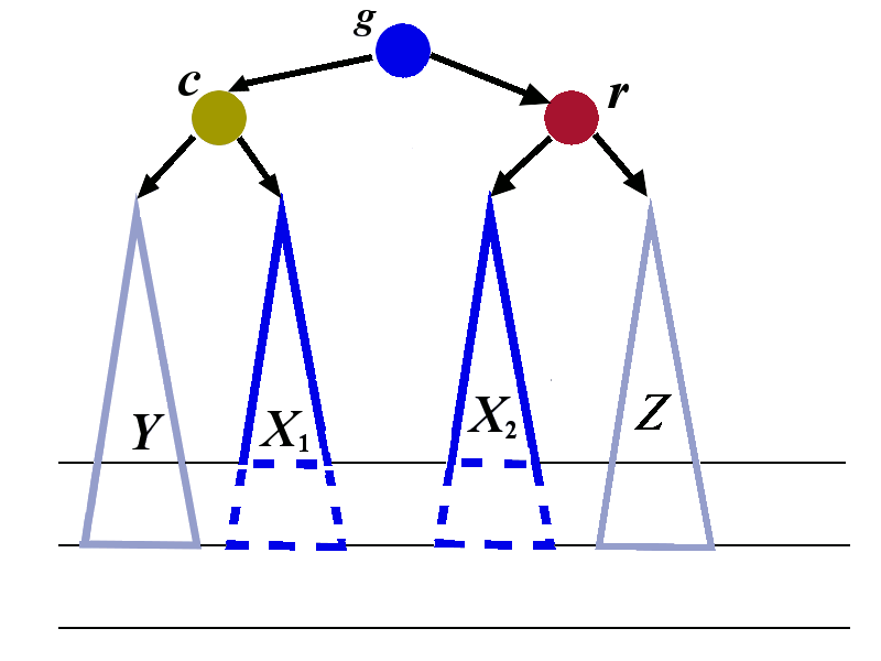
We have explained how left-right rotation restores the balance in the case when the left child has tall right sub-tree.

An analogous right-left rotation is used to restore the balance in the case when the right child has tall left sub-tree.

5. Problems

Problem 1. The node of the binary tree is defined in the following way

class TN{
public:
    long content;
    TN* aLeft;
    TN* aRight;
};

The implementation of the function f is given below

long f(TN* a, long h){
    if(a==nullptr){
        return 1;
    }
    long c=a->content;
    return (c%10)+(h%2)*f(a->aLeft,h+1)+(c%2)*f(a->aRight,h+1);
}

Assume that aRoot is the pointer to the root of the tree

What is the result of the evaluation f(aRoot,3)? Provide a rigorous justification for your answer.

Problem 2. What happens when the number \(55\) is inserted in the following AVL tree? What is the resulting tree after all the rotations?

Show solution

The first step in the AVL algorithm is the insertion of the number \(55\) in the binary search tree without re-balancing. The resulting tree is

The next step in the algorithm is identifying the highest node that violates the AVL property. The only such node is the root \(r\) with content \(40\). The height of its left sub-tree is 2 while the height of its right sub-tree is 4. We now denote by \(c\) the right child. The content of the node \(c\) is \(70\).

The right child has the left sub-tree of height 3 and the right sub-tree of height 2. This means that we need double rotation. We denote by \(g\) the node whose content is \(50\). The left sub-tree breaks into the tree \(X_1\) with root 45 and the tree \(X_2\) with root \(60\). The right subtree of \(c\) is denoted by \(Z\) (its root is \(95\)).

We now apply the right rotation to the node \(c\). The node \(g\) updates its pointer to the right child to contain the address of the node \(c\). The left child of \(c\) becomes the node with content \(60\). The root \(r\) of the entire tree updates its right child to point to \(g\). After this right rotation the tree becomes

The next step is the left rotation applied to the root \(r\). Its right child becomes the pointer to the node whose content is \(45\). The node with content \(50\) updates its left child to point to the original root. The node with content \(50\) becomes the new root. The resulting tree is shown in the picture below.